See also pure error, design matrix; or the General Linear Models, General Stepwise Regression, or Experimental Design chapters.

Lambda Prime. Lambda is defined as the geometric sum of 1 minus the squared canonical correlation, where lambda is Wilk's lambda. The squared canonical correlation is an estimate of the common variance between two canonical variates, thus 1 minus this value is an estimate of the unexplained variance. Lambda is used as a test of significance for the squared canonical correlation and is distributed as Chi-square (see below).

² = [-N -1 - {.5(p+q+1)}] * log_e

where
N    is the number of subjects
p     is the number of variables on the right
q     is the number of variables on the left

Laplace Distribution. The Laplace (or Double Exponential) distribution has density function:

f(x) = 1/(2b)*e^-|x-a|/b        - < x <

where
a     is the mean of the distribution
b     is the scale parameter
e     is the base of the natural logarithm, sometimes called Euler's e (2.71...)

The graphic above shows the changing shape of the Laplace distribution when the location parameter equals 0 and the scale parameter equals 1, 2, 3, and 4.

Latent Variable. A latent variable is a variable that cannot be measured directly, but is hypothesized to underlie the observed variables. An example of a latent variable is a factor in factor analysis. Latent variables in path diagrams are usually represented by a variable name enclosed in an oval or circle.

Layered Compression. When layered compression is used, the main graph plotting area is reduced in size to leave space for Margin Graphs in the upper and right side of the display (and a miniature graph in the corner). These smaller Margin Graphs represent vertically and horizontally compressed images (respectively) of the main graph.

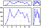
For more information on Layered Compression (and an additional example), see Special Topics in Graphical Analytic Techniques: Layered Compression.

Learning Rate in Neural Networks. A control parameter of some training algorithms, which controls the step size when weights are iteratively adjusted.

See also, the Neural Networks chapter.

Least Squares (2D graphs). A curve is fitted to the XY coordinate data according to the distance-weighted least squares smoothing procedure (the influence of individual points decreases with the horizontal distance from the respective points on the curve).

Least Squares (3D graphs). A surface is fitted to the XYZ coordinate data according to the distance-weighted least squares smoothing procedure (the influence of individual points decreases with the horizontal distance from the respective points on the surface).

Least Squares Estimator. In the most general terms, least squares estimation is aimed at minimizing the sum of squared deviations of the observed values for the dependent variable from those predicted by the model. Technically, the least squares estimator of a parameter q is obtained by minimizing Q with respect to q where:

Q = [Y_i - f_i()]²

Note that f_i() is a known function of , Y_i = f_i() + _i where i = 1 to n, and the _i are random variables, and usually assumed to have expectation of 0. For more information, see Mendenhall and Sincich (1984), Bain and Engelhardt (1989), and Neter, Wasserman, and Kutner (1989). See also, Basic Statistics, Multiple Regression, and Nonlinear Estimation.

Least Squares Means. When there are no missing cells in ANOVA designs with categorical predictor variables, the subpopulation (or marginal) means are least square means, which are the best linear-unbiased estimates of the marginal means for the design (see, Milliken and Johnson, 1986). Tests of differences in least square means have the important property that they are invariant to the choice of the coding of effects for categorical predictor variables (e.g., the use of the sigma-restricted or the overparameterized model) and to the choice of the particular generalized inverse of the design matrix used to solve the normal equations. Thus, tests of linear combinations of least square means in general are said to not depend on the parameterization of the design.

See also categorical predictor variable, design matrix, sigma-restricted model, overparameterized, generalized inverse; see also the General Linear Models or General Stepwise Regression chapters.

Left and Right Censoring. When censoring, a distinction can be made to reflect the "side" of the time dimension at which censoring occurs. Consider an experiment where we start with 100 light bulbs, and terminate the experiment after a certain amount of time. In this experiment the censoring always occurs on the right side (right censoring), because the researcher knows when exactly the experiment started, and the censoring always occurs on the right side of the time continuum. Alternatively, it is conceivable that the censoring occurs on the left side (left censoring). For example, in biomedical research one may know that a patient entered the hospital at a particular date, and that s/he survived for a certain amount of time thereafter; however, the researcher does not know when exactly the symptoms of the disease first occurred or were diagnosed.

Data sets with censored observations can be analyzed via Survival Analysis or via Weibull and Reliability/Failure Time Analysis. See also, Type I and II Censoring and Single and Multiple Censoring.

Levenberg-Marquardt algorithm. A non-linear optimization algorithm which uses a combined strategy of linear approximation and gradient-descent to locate a minimum, actively switching between the two according to the success or failure of the linear approximation: a so-called model-trust region approach (see Levenberg, 1944; Marquardt, 1963; Bishop, 1995; Shepherd, 1997; Press et. al., 1992).

See also, the Neural Networks chapter.

Levene and Brown-Forsythe tests for homogeneity of variances (HOV). A important assumption in analysis of variance (ANOVA and the t-test for mean differences) is that the variances in the different groups are equal (homogeneous). Two powerful and commonly used tests of this assumption are the Levene test and the Brown-Forsythe modification of this test. However, it is important to realize that (1) the homogeneity of variances assumption is usually not as crucial as other assumptions for ANOVA, in particular in the case of balanced (equal n) designs (see also ANOVA Homogeneity of Variances and Covariances), and (2) that the tests described below are not necessarily very robust themselves (e.g., Glass and Hopkins, 1996, p. 436, call these tests "fatally flawed;" see also the description of these tests below). If you are concerned about a violation of the HOV assumption, it is always advisable to repeat the key analyses using nonparametric methods.

Levene's test (homogeneity of variances): For each dependent variable, an analysis of variance is performed on the absolute deviations of values from the respective group means. If the Levene test is statistically significant, then the hypothesis of homogeneous variances should be rejected.

Brown & Forsythe's test (homogeneity of variances): Recently, some authors (e.g., Glass and Hopkins, 1996) have called into question the power of the Levene test for unequal variances. Specifically, the absolute deviation (from the group means) scores can be expected to be highly skewed; thus, the normality assumption for the ANOVA of those absolute deviation scores is usually violated. This poses a particular problem when there is unequal n in the two (or more) groups that are to be compared. A more robust test that is very similar to the Levene test has been proposed by Brown and Forsythe (1974). Instead of performing the ANOVA on the deviations from the mean, one can perform the analysis on the deviations from the group medians. Olejnik and Algina (1987) have shown that this test will give quite accurate error rates even when the underlying distributions for the raw scores deviate significantly from the normal distribution. However, as Glass and Hopkins (1996, p. 436) have pointed out, both the Levene test as well as the Brown-Forsythe modification suffer from what those authors call a "fatal flaw," namely, that both tests themselves rely on the homogeneity of variances assumption (of the absolute deviations from the means or medians); and hence, it is not clear how robust these tests are themselves in the presence of significant variance heterogeneity and unequal n.

Leverage values. In regression, this term refers to the diagonal elements of the hat matrix (X(X'X)^-1X'). A given diagonal element (h(_ii)) represents the distance between X values for the ith observation and the means of all X values. These values indicate whether or not X values for a given observation are outlying. The diagonal element is refered to as the leverage. A large leverage value indicates that the ith observation is distant from the center of the X observations (Neter, et al, 1985).

Life Table. The most straightforward way to describe the survival in a sample is to compute the Life Table. The life table technique is one of the oldest methods for analyzing survival (failure time) data (e.g., Berkson & Gage, 1950; Cutler & Ederer, 1958; Gehan, 1969; see also Lawless, 1982, Lee, 1993). This table can be thought of as an "enhanced" frequency distribution table. The distribution of survival times is divided into a certain number of intervals. For each interval one can compute the number and proportion of cases or objects that entered the respective interval "alive," the number and proportion of cases that failed in the respective interval (i.e., number of terminal events, or number of cases that "died"), and the number of cases that were lost or censored in the respective interval.

Based on those numbers and proportions, several additional statistics can be computed. Refer to the Survival Analysis chapter for additional details.

Line Plots, 2D. In line plots, individual data points are connected by a line.

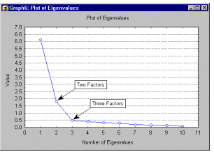
Line plots provide a simple way to visually present a sequence of values. XY Trace-type line plots can be used to display a trace (instead of a sequence). Line plots can also be used to plot continuous functions, theoretical distributions, etc.

Line Plots, 2D - Aggregrated. Aggregated line plots display a sequence of means for consecutive subsets of a selected variable.

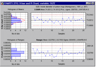
You can select the number of consecutive observations from which the mean will be calculated and if desired, the range of values in each subset will be marked by the whisker-type markers . Aggregated line plots are used to explore and present sequences of large numbers of values.

Line Plots, 2D (Case Profiles). Unlike in the regular line plots where the values of one variable are plotted as one line (individual data points are connected by a line), in case profile line plots, the values of the selected variables in a case (row) are plotted as one line (i.e., one line plot will be generated for each of the selected cases). Case profile line plots provide a simple way to visually present the values in a case (e.g., test scores for several tests).

Line Plots, 2D - Double-Y. The Double-Y line plot can be considered to be a combination of two separately scaled multiple line plots. A separate line pattern is plotted for each of the selected variables, but the variables selected in the Left-Y list will be plotted against the left-Y axis, whereas the variables selected in the Right-Y list will be plotted against the right-Y axis (see example below). The names of all variables will be identified in the legend with the letter (R) for the variables associated with the right-Y axis and with the letter (L) for the variables associated with the left-Y axis.

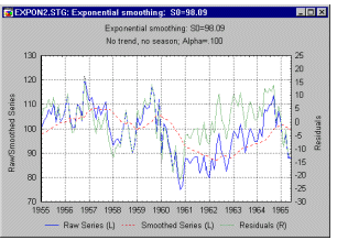
The Double-Y line plot can be used to compare sequences of values of several variables by overlaying their respective line representations in a single graph. However, due to the independent scaling used for the two axes, it can facilitate comparisons between otherwise "incomparable" variables (i.e., variables with values in different ranges).

Line Plots, 2D - Multiple. Unlike regular line plots in which a sequence of values of one variable is represented, the multiple line plot represents multiple sequences of values (variables). A different line pattern and color is used for each of the multiple variables and referenced in the legend.

This type of line plot is used to compare sequences of values between several variables (or several functions) by overlaying them in a single graph that uses one common set of scales (e.g., comparisons between several simultaneous experimental processes, social phenomena, stock or commodity quotes, shapes of operating characteristics curves, etc.).

Line Plots, 2D - Regular. Regular line plots are used to examine and present the sequences of values (usually when the order of the presented values is meaningful).

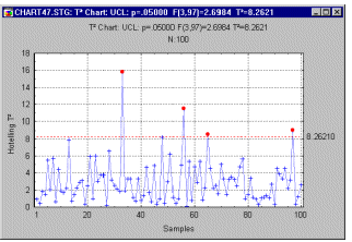
Another typical application for line sequence plots is to plot continuous functions, such as fitted functions or theoretical distributions. Note that an empty data cell (i.e., missing data) "breaks" the line.

Line Plots, 2D - XY Trace. In trace plots, a scatterplot of two variables is first created, then the individual data points are connected with a line (in the order in which they are read from the data file). In this sense, trace plots visualize a "trace" of a sequential process (movement, change of a phenomenon over time, etc.)

Linear (2D graphs). A linear function (e.g., Y = a + bX) is fitted to the points in the 2D scatterplot.

Linear (3D graphs). A linear function (e.g., Y = a + bX) is fitted to the points in the 3D scatterplot.

Linear Activation function. A null activation function: the unit's output is identical to its activation level.

See also, the Neural Networks chapter.

Linear Modeling. Approximation of a discriminant function or regression function using a hyperplane. Can be globally optimized using "simple" techniques, but does not adequately model many real-world problems.

See also, the Neural Networks chapter.

Linear Units. A unit with a linear PSP function. The unit's activation level is the weighted sum of its inputs minus the threshold - also known as a dot product or linear combination. The characteristic unit type of multilayer perceptrons. Despite the name, a linear unit may have a non-linear activation function.

See also, the Neural Networks chapter.

Link Function and Distribution Function. The link function in generalized linear models specifies a nonlinear transformation of the predicted values so that the distribution of predicted values is one of several special members of the exponential family of distributions (e.g., gamma, Possion, binomial, etc.). The link function is therefore used to model responses when a dependent variable is assumed to be nonlinearly related to the predictors.

Various link functions (see McCullagh and Nelder, 1989) are commonly used, depending on the assumed distribution of the dependent variable (y) values:
Normal, Gamma, Inverse normal, and Poisson distributions:

Identity link:	f(z) = z
Log link:	f(z) = log(z)
Power link:	f(z) = za,	for a given a

Binomial, and Ordinal Multinomial distributions:

Logit link:	f(z)=log(z/(1-z))
Probit link:	f(z)=invnorm(z)	where invnorm is the inverse of the standard normal cumulative distribution function.
Complementary log-log link:		f(z)=log(-log(1-z))
Loglog link:	f(z)=-log(-log(z))

Multinomial distribution:

Generalized logit link:

f(z1|z2,…,zc)=    log(x1/(1-z1-…-zc))

where the model has c+1 categories.

For discussion of the role of link functions, see the Generalized Linear Models chapter.

Local Minima. Local "valleys" or minor "dents" in a loss function which, in many practical applications, will produce extremely large or small parameter estimates with very large standard errors. The Simplex method is particularly effective in avoiding such minima; therefore, this method may be particularly well suited in order to find appropriate start values for complex functions.

Logarithmic Function. This fits to the data, a logarithmic function of the form:

y = q*[log_n(x)] + b

Logistic Distribution. The Logistic distribution has density function:

f(x) = (1/b)*e^-(x-a)/b * [1+e^-(x-a)/b]^-2

where
a     is the mean of the distribution
b     is the scale parameter
e     is the base of the natural logarithm, sometimes called Euler's e (2.71...)

The graphic above shows the changing shape of the Logistic distribution when the location parameter equals 0 and the scale parameter equals 1, 2, and 3.

Logistic Function. An S-shaped (sigmoid) function having values in the range (0,1). See, the Logistic Distribution.

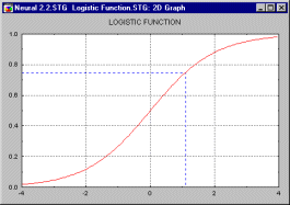
Logit Regression and Transformation. In the logit regression model, the predicted values for the dependent or response variable will never be less than (or equal to) 0, or greater than (or equal to) 1, regardless of the values of the independent variables; it is, therefore, commonly used to analyze binary dependent or response variables (see also the binomial distribution). This is accomplished by applying the following regression equation (the term logit was first used by Berkson, 1944):

y=exp(b₀ +b₁*x₁ + ... + b_n*x_n)/{1+exp(b₀ +b₁*x₁ + ... + b_n*x_n)}

One can easily recognize that, regardless of the regression coefficients or the magnitude of the x values, this model will always produce predicted values (predicted y's) in the range of 0 to 1. The name logit stems from the fact that one can easily linearize this model via the logit transformation. Suppose we think of the binary dependent variable y in terms of an underlying continuous probability p, ranging from 0 to 1. We can then transform that probability p as:

p' = log_e{p/(1-p)}

This transformation is referred to as the logit or logistic transformation. Note that p' can theoretically assume any value between minus and plus infinity. Since the logit transform solves the issue of the 0/1 boundaries for the original dependent variable (probability), we could use those (logit transformed) values in an ordinary linear regression equation. In fact, if we perform the logit transform on both sides of the logit regression equation stated earlier, we obtain the standard linear multiple regression model:

p' = (b₀ +b₁*x₁ + ... + b_n*x_n)

For additional details, see also Nonlinear Estimation or the Generalized Linear Models chapter; see also Probit Transformation and Regression and Multinomial logit and probit regression for similar transformations.

Log-Linear Analysis. Log-linear analysis provides a "sophisticated" way of looking at crosstabulation tables (to explore the data or verify specific hypotheses), and it is sometimes considered an equivalent of ANOVA for frequency data. Specifically, it allows the user to test the different factors that are used in the crosstabulation (e.g., gender, region, etc.) and their interactions for statistical significance (see Elementary Concepts for a discussion of statistical significance testing).

For more information, see the Log-Linear Analysis chapter.

Log-normal Distribution. The lognormal distribution (the term first used by Gaddum, 1945) has the probability density function:

f(x) = 1/[x(2)^1/2] * exp(-[log(x)-µ]²/2²)
0 x <
µ > 0
> 0

where
µ     is the scale parameter
   is the shape parameter
e     is the base of the natural logarithm, sometimes called Euler's e (2.71...)

The animation above shows the Log-normal distribution with mu equal to 0 for sigma equals .10, .30, .50, .70, and .90.

Lookahead in Neural Networks. For neural networks time series analysis, the number of time steps ahead of the last input variable values the output variable values should be predicted.

See also, the chapter on neural networks.

Loss Function. The loss function (the term loss was first used by Wald, 1939) is the function that is minimized in the process of fitting a model, and it represents a selected measure of the discrepancy between the observed data and data "predicted" by the fitted function. For example, in many traditional general linear model techniques, the loss function (commonly known as least squares) is the sum of squared deviations from the fitted line or plane. One of the properties (sometimes considered to be a disadvantage) of that common loss function is that it is very sensitive to outliers.

An common alternative to the least squares loss function (see above) is to maximize the likelihood or log-likelihood function (or to minimize the negative log-likelihood function; the term maximum likelihood was first used by Fisher, 1922a). These functions are typically used when fitting non-linear models. In most general terms, the likelihood function is defined as:

L=F(Y,Model)=ⁿ_i=1 { p[y_i , Model Parameters(x_i)]}

In theory, we can compute the probability (now called L, the likelihood) of the specific dependent variable values to occur in our sample, given the respective regression model.

Loss Matrix. A square matrix of coefficients multiplied by a vector of class probabilities to form a vector of cost-estimates, so that minimum-loss decisions can be made.

See also, the chapter on neural networks.

LOWESS Smoothing (Robust Locally Weighted Regression). Robust locally weighted regression is a method of smoothing 2D scatterplot data (pairs of x-y data). A local polynomial regression model is fit to each point and the points close to it. The method is also sometimes referred to as LOWESS smoothing. The smoothed data usually provide a clearer picture of the overall shape of the relationship between the x and y variables. For more information, see also Cleveland (1979, 1985).