Consumer theory: indifference curves

We've set up the consumer's constraints which establish consumption possibilities
Now we turn to preferences to see what choices the consumer will make

Focus is on pure consumption: use it or lose it, but you have free disposability (you can throw away but not sell what you don't consume)

    For any bundles A and B, a consumer is able to decide:
    "I prefer A to B."
    "I prefer B to A."
    "I am indifferent between A and B."

    Concept related to total utility: Marginal Utility (MU): the increase in total utility due to the consumption of one extra unit of some item, holding all else constant:
    MUx = DU/DX
    MUy = DU/DY

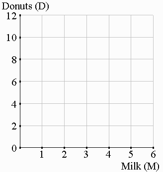
Example: You consume donuts (D) and milk (M).
Milk consumption rises with your quantity of donuts fixed

Property (1) of utility: the MU of any economic good is positive.
MUx > 0. (more is better)

Property (2) of utility: MU falls as consumption rises
("law of diminishing marginal utility)."

As with the budget line for consumer constraints, to illustrate consumer decisionmaking for more than one item, we need to be able to incorporate consumer utility into our x-y diagram. That's our next step.

Indifference curves: Arise when consumers face a choice and respond, "I don't care which I choose."
Indifference curve: a set of consumption bundles that a consumer regards as equally desirable.

Example: milk and donuts.

Along the indifference curve,
U(M,D) = Uo,
where Uo is a constant.

? Where in the diagram are consumption bundles that you would not like as much as the bundles along Uo?

Bundles below Uo are less desirable to you--they have less of milk and/or donuts than the points along Uo.
Note that a single indifference curve divides up an entire consumption set into more preferred and less preferred consumption bundles.

Indifference map: a set of several indifference curves.

    Note: Utility = real income
    => all along Uo, real income is constant.
    (The consumer is equally happy even though the consumption bundles and their money costs differ.)

    Examples of indifference curves:
    Worksheet
    Think each case through and don't be surprised if these curves have rather unusual shapes compared to the 'typical' curves we covered in the basic geometry.
    Illustrations of worksheet examples (Java)

    Consider points A and B on Uo:
    Milk Donuts
A   1    10
B   2     5

    ? How has each of the following changed in the move FROM A to B?
    ? Milk consumption? DM =
    ? Donut consumption? DD =
    ? Utility? DU =

The consumer has substituted 1 glass of milk for 5 donuts and is just as well off as before.
In general, the slope of an indifference curve tells us the rate at which good X can substitute for good Y without affecting utility.

The MRS = the maximum amount of good Y (here donuts) which a consumer is willing to give up for another unit of good X (here milk).
Geometry: MRS= the size of the slope of an indifference curve.

Now let's take a closer look at the slope of a typical indifference curve, the curve's marginal rate of substitution.

Recall: Px and Py determine the slope of the BL (OppCost)
The analogy here: MUx and MUy determine the slope of Uo

Even though we can’t directly measure MUs, we can show that they do determine the slope of Uo.

    Rearrange terms:
        |-DY|      MUx
        -------- = -------- ( = MRS)
        | DX|     MUy

General case:	\|	Example here:
MUx = utility gained from an extra X	\|	MUx = 10 utils
MUy = rate utility falls when giving up Y	\|	MUy = 2 utils
	\|
=> MUx/MUy	\|	10u/(2u per Y)
= total Y you can give up for 1X w/o losing utility	\|	5Y for 1X
= \|-DY/DX\| (the size of the slope of Uo)	\|

The more satisfying (i.e., valuable) milk is compared to donuts, the more donuts a consumer will give up to get that milk.
So Uo will be steep when milk is valued highly compared to donuts, flat when milk is not so highly valued compared to donuts.

    Summary: comparing BL and Uo
    Slope of BL reflects the price of X relative to Y
    Slope of Uo reflects the value of X relative to Y

Property (1): Every consumption point is on some indifference curve.
(Indifference curves can be "thick"--for example, if you don't consume either item)

Property (2): Indifference curves for economic goods slope down.
(reflects your willingness to trade off items you like)

? Would an individual's indifference curves surprise you if they looked like the ones shown here?
? Why or why not?

? What property could we state to avoid this problem?

Property (3): An individual's indifference curves never cross.

The last property pertains to the curvature of Uo:

Property (4): Indifference curves for goods are convex to the origin.

    To see why, consider the following four points along Uo:
Point  Milk Donuts
    A      1    10
    A'     2     5
    B      4     2.5
    B'     5     2

    At point A you have lots of donuts and little milk (1,10).
    At A: You place a high value on more milk (MRS=5)
    (5D for 1M, moving you to point A').

    At B, you have more milk and fewer donuts.
    At B: You place a lower value on even more milk (MRS=0.5)
    (1/2D for 1M, moving you to point B').

So notice that the marginal value you place on a good depends on how much you already have.

    The econ version of the relativity theory of value: Examples:
            diamond/water paradox
            beads for manhattan
            frequency of a 3d child (56% for (0,2) v. 51% for (1,1))

The 2 limits to indifference curve convexity are (1) perfect complements and (2) perfect substitutes

    Ordinarily, we have smooth, convex downward-sloping indifference curves.
    For specificity, what sort of utility function would give us that result?
    One common one is...

The most commonly used utility function: Cobb-Douglas utility function:
U = a^.X^BxY^By

    Key result: For a Cobb-Douglas utility function:
                       Bx     Y
          MRS = ---- ^. ---
                       By     X

which falls continuously as we move down an indifference curve (X falls and Y rises).

Numerical example:
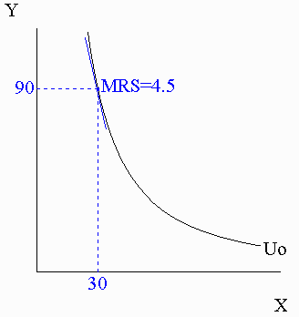
U = X^0.6·Y^0.4

? MRS formula =

If Y=90 and X=30:
? MRS value =