WILLINGNESS TO PAY AND THE DEMAND CURVE
Measuring Willingness to Pay and Marginal Benefit
Suppose we asked an individual who is consuming a zero amount of good X, "How much money would you be willing to pay for one unit of X?" Because the money, which the individual would pay, can be used to buy all other goods, not just one good, the question implicitly asks the individual to compare X with all other goods. In general, the answer to this question would depend on how much utility would increase with one unit of X and on how much utility would decrease because less would be spent on other goods given the budget constraint. In other words, the answer would depend on the person's preferences for X and all other goods as represented by utility.
Suppose that the answer is $5. Let
us assume that the answer to the question gives us the true measure of
the consumer's preferences. Then, once we get an answer to the first question,
we could ask, "How much would you be willing to pay for two units of X?"
Again, the answer would depend on how much utility would increase with
another unit of X and on how much utility would decrease with less to spend
on other goods. Suppose the answer is, "I would be willing to pay $8? We
could then continue to ask the consumer about more and more units of X.
We summarize the hypothetical answers in Table 5.6. The column labeled
"Willingness to Pay" tabulates the answers to the question.
| Quantity of X | Willingness to Pay for X (benefit from X) | Marginal Benefit from X |
| 0 | $0.00 | --- |
| 1 | $5.00 | $5.00 |
| 2 | $8.00 | $3.00 |
| 3 | $9.50 | $1.50 |
| 4 | $10.50 | $1.00 |
| 5 | $11.00 | $.50 |
This method of obtaining information about people's preferences is sometimes used in practice. For example, a recent survey of people in the United States endeavored to obtain information about people's preferences for the 1.3 million-acre Sclway Bitterroot Wilderness area in northern Idaho versus other goods. The survey question read, "If you could be sure the Sclway Bitterroot Wilderness would not be opened for the proposed timber harvest and would be preserved as a 'wilderness area' indefinitely, what is the most that your household would pay each year through a federal income tax surcharge designated for preservation of the Sclway Bitterroot Wilderness?" In this example, X is the "wilderness area."
But the answers to such questions are not always reliable, and economists prefer to estimate people's willingness to pay by looking at their decisions to purchase goods at different prices in the market. Regardless of how information about people's willingness to pay is obtained, willingness to pay provides a useful dollar measure of the benefits people receive from consumption.
Graphical Derivation of the Demand Curve
A demand curve can be derived from the information about willingness to pay and marginal benefit of X in Table 5.6. Suppose that X is raisins (rice, salt, tea, orange juice, CDs, movies, or any other good will serve just as well as an example). We want to ask how many pounds of raisins the person would buy at different prices. We imagine different hypothetical prices for raisins from astronomical levels like $7 a pound to bargain basement levels like $.50 a pound.
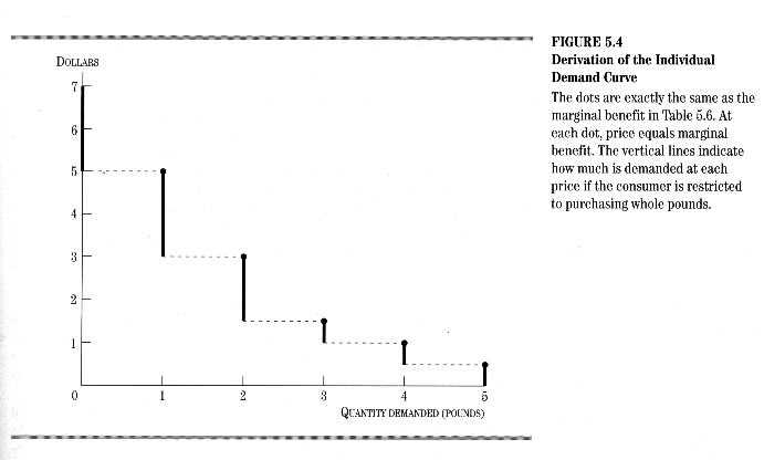
To proceed graphically, we first plot the marginal benefit from Table 5.6 in Figure 5.4. Focus first on the black dots in Figure 5.4. The lines will be explained in the next few paragraphs. The horizontal axis in Figure 5.4 measures the quantity of raisins. On the vertical axis we want to indicate the price as well as the marginal benefit, so we measure the scale of the vertical axis in dollars. The black dots in Figure 5.4 represent the marginal benefit an individual gets from consuming different amounts of raisins.
How many pounds of raisins would this person consume at different prices for raisins? First suppose that the price is very high----$7 a pound. Draw an arrow pointing to this $7 price in Figure 5.4. We are going to derive a demand curve for this individual by gradually lowering the price from this high value and seeing how many pounds would be purchased at each price. As the price declines, you can slide your arrow down the vertical axis. For each price we ask the same question: how many pounds would the person buy? To make things simple at the start, assume that the person buys only whole pounds of raisins. You might want to imagine that the raisins come in 1-pound cellophane packages. We consider fractions of pounds later.
Suppose then that the price is $7 a pound. The marginal benefit from 1 pound of raisins is $5. Thus, the price is greater than the marginal benefit. Would the person buy a pound of raisins at this price? Because the price the consumers would have to pay is greater than the marginal benefit, the answer would be no: the person would not buy a pound of raisins at a price of $7. If the minimum amount of raisins that can be purchased is 1 pound, then the person will buy no pounds at a price of $7 per pound. The person might buy something else like a magazine, but we know that no raisins will be consumed. We have shown, therefore, that the quantity demanded of raisins is zero when the price is $7.
Continue to lower the price. As long as the price is more than $5, the person will not buy any raisins. Hence. the quantity demanded at all prices higher than $5 is zero. We indicate this by the red line on the vertical axis above the $5 mark.
Now watch what happens when the price drops to $5. The marginal benefit from a pound of raisins is $5 and the price is $5. Now will a pound of raisins be purchased? Yes, because the marginal benefit from raisins is just equal to the price. Hence, the quantity demanded increases to I pound when the price falls to $5. In Figure 5.4, the quantity demanded when the price is $5 is given by the black dot at I pound.
Continue lowering the price, slipping the arrow down the axis. The quantity demanded will stay at I pound as long as the price remains above the marginal benefit of buying another pound of raisins, or $3. We therefore extend the red line down at I pound as the price falls from $5 down to $3. Consider, for example, a price of $4. The person has already decided that I pound will be bought and the question is whether a second pound of raisins is worthwhile. Another pound has a marginal benefit of $3 (willingness to pay goes from $5 to $8 as the quantity increases from I to 2 pounds). The person has to pay $4, which is more than the marginal benefit. Hence, the quantity demanded stays at 1 pound when the price is $4. However, when the price falls to $3, another pound is purchased. That is, when the price is $3, the quantity demanded is 2 pounds, which is shown graphically by the black dot at 2 pounds.
Now suppose the price falls below $3, perhaps to $2. Is a third pound purchased? The marginal benefit of a third pound is $1.50; is it worth it to buy a third pound at $2 per pound? No. The quantity demanded stays at 3 pounds when the price is between $3 and $1.50, ,which we denote by extending the red line down from the black dot at 2 pounds. This story can be continued. As the price continues to fall, more pounds of raisins are demanded.
By considering various prices from over $5 to under $.50, we have traced out an individual demand curve that slopes downward. As the price is lowered, more raisins are purchased. The demand curve is downward-sloping because of diminishing marginal benefit. At each black dot in the diagram, price equals the marginal benefit.
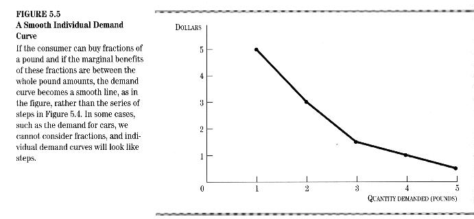
The jagged shape of the demand curve in Figure 5.4 may look strange. It is due to the assumption that only 1-pound packages of raisins are considered by the consumer. In the case of raisins, it is usually possible to buy fractions of a pound, and if the marginal benefit of the fractions are between the values of the whole pounds, then the demand curve will be a smooth line, as shown in Figure 5.5. Then price would equal marginal benefit not only at the black dots but also on the lines connecting the dots. If you are unsure of this, imagine creating a new Table 5.1 and Figure 5.4 with utility for each ounce of raisins. There will be a point at each ounce and with 16 ounces per pound there will be so many points that the curve will be as smooth as Figure 5.5.
The Price Equals Marginal Benefit Rule
We have discovered another important
principle of consumer behavior. If the consumer can adjust consumption
of a good in small increments--such as fractions of a pound--then the consumer
maximizes utility by buying an amount for which the price equals marginal
benefit. This condition can be applied to any good--movies, apples,
peanuts, comic books--not just raisins.
Review
CONSUMER SURPLUS
In many cases people are willing to pay more for an item consumed than they have to pay for it. You may love going to see your favorite movie and would be willing to pay five times the $6 admission price to see it. But just like everyone else in line, you pay only $6 even if it is worth $30 to you. The difference between the $30 and the $6 is called consumer surplus.
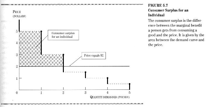
In general, consumer surplus is the difference between the willingness to pay for an additional item (say $30 for a movie)--its marginal benefit--and the price paid for it (say $6 for a movie). Suppose the price of raisins is $4 per pound. Then the consumer in our previous example purchases 1 pound and the marginal benefit of the pound is $5. In that situation the consumer gets a consumer surplus because the marginal benefit of the raisins to the consumer is $5 but the price paid is only $4 per pound. Consumer surplus is the difference, or $1. If the price were $3.50, then the consumer surplus would be greater, or $1.50.
Suppose the price falls further so that two items are purchased. Consumer surplus is then defined as the sum of differences between the marginal benefits of each item and the price paid for the item. For example, if the price per pound of raisins is $2, as in Figure 5.7, then 2 pounds of raisins will be purchased and the consumer surplus will be $5 - $2 = $3 for the first pound plus $3 - $2 = $1 for the second pound for a total of $4. That is, the consumer surplus is $4.
Figure 5.7 shows graphically how consumer surplus is the area between the demand curve and the line indicating the price. In Figure 5.7 the total shaded area is equal to 4, consisting of two rectangular blocks, one with an area of 3 and the other with an area of 1. The area is the extra amount that the consumer is getting because the market price is lower than what the consumer is willing to pay.
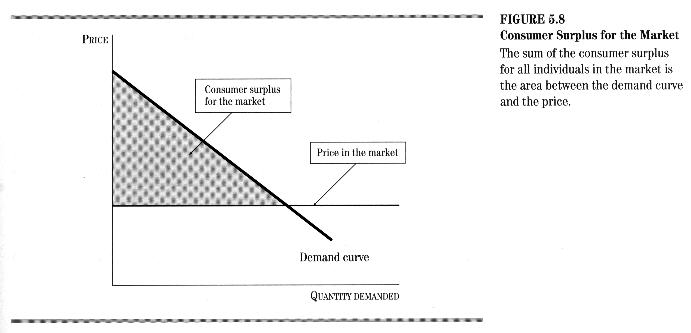
There is also consumer surplus for the entire market. It is the sum of the consumer surpluses of all individuals who have purchased goods in the market. This can be illustrated with the market demand curve, as in Figure 5.8. It is the area between the market demand curve and the market price line.
Consumer surplus has many uses in economics. It is used to measure how well the market system works. We will show in Chapter 6 that the market system maximizes consumer surplus under certain circumstances.
Consumer surplus can also be used to measure the gains to consumers that come from an innovation. For example, if a new production technique lowers the price of raisins, then the consumer surplus will increase: the area between the demand curve and the market price line increases. This increase is a measure of how much the new technique is worth to society.
Consumer surplus is also used to evaluate the benefits of government policies, such as building a new bridge or creating a new wilderness area. These policies will increase or decrease consumer surplus, and their value to society can be estimated using the concept of consumer surplus.
Review