Supply and Demand geometry for the trade market
The trade market depicts transactions
that occur between large trading partners. When large partners trade, their
transactions set equilibrium world prices that depend on how much the countries
end up trading with each other. The supply and demand curves specific to the
trade
market are:
Dm = the demand for imports by the
buying country, and
Sx = the supply of exports by the selling country.
To illustrate how the market works, consider the possibility of beer
trade between the U.S. and Germany.
Step1: Find each country's autarky (no trade) equilibrium based on
the country's domestic supply and
demand conditions. The country with the higher autarky price (Pa)
-- the U.S. in this example will demand imports of beer with trade, and the
country with the lower Pa (Germany) will supply exports of beer. The
equilibrium trade price will end up somewhere between the U.S. and
German autarky prices.
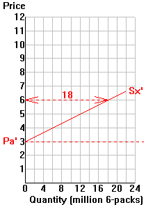
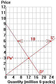
Step2: Plot the U.S. import demand curve (Dm by US)
and Germany's export supply curve (Sx by Ger) in the trade
market. Here are the formulas for plotting each of the curves:
Dm: For any price below the
importer's Pa, quantity demanded of imports, Qm = Qd - Qs.
(Table column d)
Sx: For any price above the
exporter's Pa, quantity supplied of exports, Qx = Qs
- Qd
. (Table column h)
Step 3: Use the Dm and Sx curves
in the trade market to determine the equilibrium trade price and
quantity traded.
To do: (1) Derive the Qm data and plot Dm for the
U.S. (Germany has already been completed.)
(2) With free trade, the equilibrium price for
beer = $______, and the equilibrium quantity traded = ______
million 6-packs.
| U.S. |
|
Germany (') |
| Domestic market |
Trade market |
|
Domestic market |
Trade market |
| a |
b |
c |
d |
|
e |
f |
g |
h |
| P |
Qd |
Qs |
Qm (imported) |
|
P |
Qd |
Qs |
Qx (exported) |
| 7.00 |
8 |
11 |
Not relevant |
|
7.00 |
4 |
28 |
24 |
| 6.00 |
10 |
10 |
______ |
|
6.00 |
6 |
24 |
18 |
| 5.00 |
12 |
9 |
______ |
|
5.00 |
8 |
20 |
12 |
| 4.00 |
14 |
8 |
______ |
|
4.00 |
10 |
16 |
6 |
| 3.00 |
16 |
7 |
______ |
|
3.00 |
12 |
12 |
0 |
| 2.00 |
18 |
6 |
______ |
|
2.00 |
14 |
8 |
Not relevant |
|
|
|