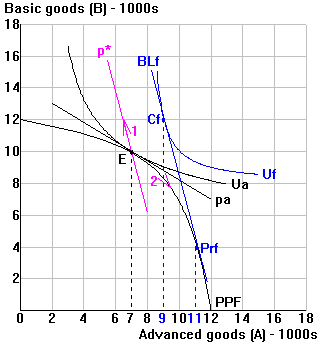
General Equilibrium Geometry of Autarky and Free Trade: Recap

    Before trade (ignore everything in the diagram labeled "f"):
        Production point: E
        Consumption point: E
        Domestic relative price and cost: pa
        Utility: Ua

    The incentive to trade: Given a global relative price = p* (>pa), notice the incentive to exchange and to specialize:
    Arrow 1 illustrates the incentive to exchange: the economy can move into the region of more preferred consumption bundles by exporting A in exchange for B, moving left/up along p*.
    Arrow 2 illustrates the incentive to specialize: the economy can move to a higher budget line by increasing production of A and reducing production of B, moving right/down along its PPF.

    Specialization occurs until the economy reaches its highest attainable budget line, BLf at production point Prf. At that point, the relative cost of the two goods (slope of PPF) = the global relative price ratio (slope of BLf).
    Exchange occurs until the economy reaches its highest attainable indifference curve (Uf), at consumption point Cf on BLf. At that point the relative value of the two goods (slope of Uf) = the global relative price ratio (slope of BLf).

    With free trade:
        Production point: Prf
        Consumption point: Cf
        Domestic relative price and cost: pf
        Utility: Uf