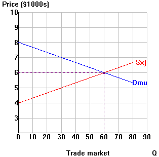
| Example: Consider the trade market for small trucks exported from Japan (J) to the U.S. (U), illustrated in the trade-market diagram below: | |||||||||||||||||
 |
|||||||||||||||||
| A. Basic geometry: Suppose the U.S. imposes a $2,000 tariff on small trucks imported from Japan. | |||||||||||||||||
| Step 1: Shift Sxj up by the amount of the tariff (tar);
label your new dotted-line curve Sx+tar. Step 2: Use Sx+tar to find the new equilibrium quantity traded (Q'). Step 3: Go up to the import demand curve at Q' to find the new price in the U.S. (Pu') Step 4: Go up to the export supply curve at Q' to find the the new price in Japan (Pj'). Step 5: Indicate where the U.S. tariff revenue shows up in the diagram. |
|||||||||||||||||
| B. Analysis: Comparing the tariff to free trade. 1. Price effects: |
|||||||||||||||||
| The "trade price" (Ptr) is the price which the
importing country actually pays to the exporting country. How high is Ptr with free trade? ______ With the U.S. tariff? ______ |
|||||||||||||||||
| 2. Welfare effects: | |||||||||||||||||
|
|||||||||||||||||