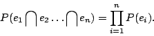
A random variable is a measurable function ![]() , where S is a set,
, where S is a set, ![]() is a sigma-algebra on S, and
is a sigma-algebra on S, and ![]() is a measure defined on
is a measure defined on ![]() such that
such that ![]() . The set M is a metric space in general.
Usually it is
. The set M is a metric space in general.
Usually it is ![]() or a subset thereof. The triple
or a subset thereof. The triple ![]() is called a ``probability space''.
is called a ``probability space''.
A random variable induces a measure, ![]() on the target space, M. This is called
the ``distribution of X''.
on the target space, M. This is called
the ``distribution of X''.
All of this is more formal and general than what we shall need for this
course. ![]() is usually written as P, or Pr; a
shorthand for ``probability''. S is often finite, in which case
is usually written as P, or Pr; a
shorthand for ``probability''. S is often finite, in which case ![]() is the collection of all subsets of S. In
this case, it suffices to define P for all
is the collection of all subsets of S. In
this case, it suffices to define P for all ![]() . S could be countably infinite, as in the
non-negative integers. Finally, S could be
. S could be countably infinite, as in the
non-negative integers. Finally, S could be ![]() , or an interval such as [0,1] or
, or an interval such as [0,1] or ![]() . In this case, the measure is often expressed in
terms of a ``density function'', f. Thus
. In this case, the measure is often expressed in
terms of a ``density function'', f. Thus ![]() .
.
Independence
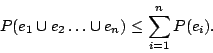
An event is a subset of S or M. Events ![]() are called ``independent'' if
are called ``independent'' if
Note that equation 1 is
written for events in S. If the ei were events
in M, we would write
Random variables are called independent if equation 2 holds
for any collection of subsets of M. When events or random variable are
independent, people often say that ``they have nothing to do with one another''.
This is imprecise. A better way to think about independence is to think
``product measure''. Random variables ![]() are called i.i.d. (independent and
identically distributed) if they all have the same distribution and if any
finite collection are independent.
are called i.i.d. (independent and
identically distributed) if they all have the same distribution and if any
finite collection are independent.
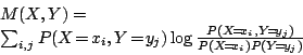
Examples of independence and non-independence
EXAMPLE 1 X and Y are discrete random variables on the same space. The set of all possibilities for the values of X and Y are given in Table 1.
|
How can we prove that X and Y are independent in Table 1. It's simple. If
pi,j is the probability in row i and
column j, then ![]() .
.
EXAMPLE 2 X and Y are discrete random variables on the same space. A new set of all possibilities for the values of X and Y are given in Table 2.
|
How can we prove that X and Y are not independent in Table 2. Again, it's simple. Find a counterexample. For example, P(X = 7) = 0.233 and P(Y = 6) = 0.25. The product of these numbers is 0.05825 which is not equal to 0.05.
Mutually exclusive events
This concept is easier than that of independence. Events ![]() are called ``mutually exclusive''
are called ``mutually exclusive'' ![]() . In this case,
. In this case,
Note that equation 3
does not imply mutually exclusive events, since some events can have probability
0. In general,
Conditional probability and
Bayes Theorem
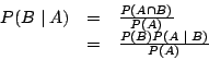
If A and B are events, then we define the ``conditional
probability of A given B'', ![]() by
by
Bayes theorem (This bit of trivia should really be called ``Bayes lemma'' at best. Bayes was a very minor figure in probability theory and certainly doesn't deserve to have his name used so often.)
Equation 5 can
be rewritten as:
From this, it is easy to derive:
Example: Using Bayes Theorem
General Widgets (GW) is a company that manufactures widgets. Each widget needs 3 doodles. The doodles are manufactured by 4 different companies, C1, C2, C3 and C4. 10% of C1's doodles are defective, 5% of C2's doodles are defective, 2% of C3's doodles are defective and 1% of C4's doodles are defective. Because of price and availability, 40% of GW's doodles come from C1, 30% come from C2, 20% from C3 and the final 10% from C4. A widget fails if any one of its doodles is defective. The failures are independent of one another.
We first need to answer the question: ``What is the probability that a randomly selected doodle is defective?''
Let D be the event that a doodle is defective. Let
Ci be the event that company Ci produces a doodle, ![]() . Then:
. Then:
| P(D) | = | 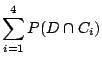 |
|
| = | 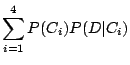 |
||
| = | |||
| = | 0.06 |
If a doodle is defective, what is the probability that it was made by C1?
| P(C1 | D) | = | 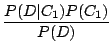 |
|
| = | |||
| = |
Mean, variance and characteristic functions
For a real valued random variable, X, we define its ``expectation'',
or ``expected value'' as
| (8) |
| (9) |
| (10) |
The nth moment of X ``about the mean is
defined by
| (11) |
The ``characteristic function'', ![]() , is defined by
, is defined by
| (12) |
What good are characteristic functions? 1. ![]() have the same distribution
have the same distribution ![]()
2. If ![]() are independent and
are independent and ![]() , then
, then
 |
(13) |
Some important probability distributions.
BINOMIAL DISTRIBUTION
Apart from the trivial case where X = 0 with probability 1, the
simplest case of a random variable is one that takes on just 2 values. These are
often taken as 0 and 1, although -1 and +1 are sometimes used. Sometimes, we
might write ``heads'' and ``tails'' for the 2 possibilities, indicating that
X represents the results of a coin toss. We'll adopt the following
convention. X takes on the 2 values, 1 and 0 with probabilities p
and q respectively, where p + q = 1. Let ![]() , where the Xi are
independent copies of X. What is the distribution of Y. Clearly
Yn can take on any value between 0 and n. In
fact, simple combinatorics gives us:
, where the Xi are
independent copies of X. What is the distribution of Y. Clearly
Yn can take on any value between 0 and n. In
fact, simple combinatorics gives us:
| (14) |
POISSON DISTRIBUTION
Suppose that p is ``small'' and the ``n'' is large. To be more
explicit, let's set ![]() and see what happens as
and see what happens as ![]() . Stirling's formula gives the limiting value for
P(Yn = k) as
. Stirling's formula gives the limiting value for
P(Yn = k) as ![]() . The characteristic function is
. The characteristic function is ![]() . It's easier to do this limiting process in
``reciprocal space''. First,
. It's easier to do this limiting process in
``reciprocal space''. First, ![]() . Thus
. Thus ![]() . This approaches
. This approaches ![]() as
as ![]() .
.
This limiting distribution is called the ``Poisson distribution''. Think of it as the ``law of rare events''.
UNIFORM DISTRIBUTION
This is given by a constant density function, ![]() for
for ![]() and f(x) = 0 otherwise.
and f(x) = 0 otherwise.
GAUSSIAN DISTRIBUTION
Density is ![]() Note that
Note that ![]() and
and ![]() are the mean and variance. This is called the
``normal distribution''. The notation ``N(
are the mean and variance. This is called the
``normal distribution''. The notation ``N(![]() ,
,![]() )'' refers to this distribution. If
)'' refers to this distribution. If ![]() are i.i.d. with mean
are i.i.d. with mean ![]() and variance
and variance ![]() , then
, then
| (15) |
EXPONENTIAL AND GAMMA DISTRIBUTIONS
The density of the exponential distribution is ![]() for
for ![]() . The mean and variance are
. The mean and variance are ![]() and
and ![]() , respectively.
, respectively.
The density of the gamma distribution is given by
| (16) |
Note that ![]() yields the exponential distribution. If X
and Y are independent random variables with gamma distributions
yields the exponential distribution. If X
and Y are independent random variables with gamma distributions ![]() and
and ![]() , then X+Y has distribution
, then X+Y has distribution ![]() . Thus sums of exponential distributions give
gamma distributions with increasing parameter
. Thus sums of exponential distributions give
gamma distributions with increasing parameter ![]() .
.
GEOMETRIC DISTRIBUTION This is the discrete equivalent of the
exponential distribution. ![]() for some constant
for some constant ![]() , q = 1 - p. A simple calculation
shows that
, q = 1 - p. A simple calculation
shows that ![]() .
.
INFORMATION CONTENT:
ENTROPY AND RELATIVE
ENTROPY
For a random variable, X with discrete probability values pi = P(X
= xi) the ``entropy'' is defined by ![]() . The sum is replaced by an integral for
non-discrete probabilities. Since
. The sum is replaced by an integral for
non-discrete probabilities. Since ![]() , there is no problem in taking ``
, there is no problem in taking ``![]() '' to be 0. Also, the general
'' to be 0. Also, the general ![]() is written here. In statistical mechanics
applications, it is natural to take the natural logarithm. For molecular
sequence analysis, base 2 is appropriate and the entropy is then said to be
expressed ``bits''. In any case, the choice of base only changes the result by a
constant scale factor.
is written here. In statistical mechanics
applications, it is natural to take the natural logarithm. For molecular
sequence analysis, base 2 is appropriate and the entropy is then said to be
expressed ``bits''. In any case, the choice of base only changes the result by a
constant scale factor.
If X takes on finitely many values, n, a trite calculation
using Lagrange multipliers shows that H(X) is maximized when ![]() . In this case, the entropy is
. In this case, the entropy is ![]() . Entropy is maximized when the distribution is
``most spread out''. Also, note that this spread out distribution is increasing
with the number of states.
. Entropy is maximized when the distribution is
``most spread out''. Also, note that this spread out distribution is increasing
with the number of states.
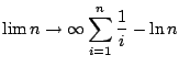
Entropy was used by Shannon in his effort to understand information content
of messages. Let's consider the following problem. We're receiving a message
that's been encoded into bits (0's and 1's). If there were no noise (no error)
at all, we would have 1 bit of information per bit received. Think of the signal
as Yi + Xi.
Yi is the pure signal with no error. It is
``deterministic''. Xi is the ``random error''. It is 0
(no error) with probability p and 1 (bit swap error) with probability
1-p. The entropy is ![]() . This approaches 0 as
. This approaches 0 as ![]() . That is, small p implies small error.
For p = 1/2, the entropy is
. That is, small p implies small error.
For p = 1/2, the entropy is ![]() in bits. That is, all information is lost. Note
that p = 1 is useful, since we can simply swap bits.
in bits. That is, all information is lost. Note
that p = 1 is useful, since we can simply swap bits.
In this course, we will be computing entropy for ``sample distributions''.
For 2 random variables, X and Y, define the ``relative
entropy'' of X with respect to Y as
| (17) |
Finally we define the ``mutual information'' of X with respect to Y as
 |
(18) |
Mutual information is the relative entropy of the joint probability distribution of X and Y and the product distribution. As such, it is a good measure of the independence of X and Y.
Coin tossing and longest runs
Infinite tossing of a consistent coin.
Let ![]() be a series of i.i.d. random variables
such that
be a series of i.i.d. random variables
such that ![]() and
and ![]() , where 0 < p < 1 and q = 1
- p. X is 1 for a head and is 0 for a tail.
, where 0 < p < 1 and q = 1
- p. X is 1 for a head and is 0 for a tail.
We want to look at this series in a novel way. Let Ri be the length of the ith ``run of heads'', to be called ``run'' henceforth. By definition, a run begins at the first position, or at the first position after a T. A run ends when as soon as a T is encountered. The length of a run is the number of heads in the run. The tail is not counted. This means that we are including runs of zero length.
Another way of stating this is by defining Bi to be the beginning index of the ith run. Then B1 = 1 by definition and Bi = Bi-1 + Ri-1 + 1 for i > 0. Note that R1 = 0 if X1 = T.
The beginnings of runs for a particular sequence of coin tosses are shown below using the symbol |.
     2   4   6   8  10  12  14  16
   T T H H H T H H H H T T H T T H H ...
   | | |       |         | |   | |
| i | 1 | 2 | 3 | 4 | 5 | 6 | 7 | 8 | |
| Bi | 1 | 2 | 3 | 7 | 12 | 13 | 15 | 16 | |
| Ri | 0 | 0 | 3 | 4 | 0 | 1 | 0 | ? |
The sequence of heads and tails are independent, and the new sequence of runs, each one ending with a tail, are also independent. This means that the random variables, Ri, are independent. particular, the Ris are not independent. In a sequence of finite length, n, we cannot say when the last run ends unless Xn = 0.
What is the distribution of the Ris? They have a
common distribution. In fact, ![]() . That is, Ri + 1 has
the geometric distribution with parameter q. Ri
+ 1 is the number of tosses until a T is encountered.
. That is, Ri + 1 has
the geometric distribution with parameter q. Ri
+ 1 is the number of tosses until a T is encountered.
In particular,
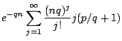
The expectation is given by
We can now very easily answer the question ``What is the expected number of
runs of any particular size in n tosses?''. A run of size k may
begin anywhere with the same probability
q2pk, except for the first position.
In any case, the expected number of runs is simply
q2pk(n-k+1). If we let
![]() and think of n as ``large'', then:
and think of n as ``large'', then:
Using a fixed number of coin tosses, n, results in run lengths that are not independent and that do not end cleanly at n. We will now replace the coin toss by a ``Poissonized version'' that has much better properties and that approximates the true coin toss sufficiently well for our conclusions to transfer.
Let ![]() be a series of i.i.d. random variables
with the common ``run'' distribution discussed above (equations 19
& 20).
Let N be a Poisson random variable independent of the R's and with
mean nq. Consider the ``Poissonized'' coin toss:
be a series of i.i.d. random variables
with the common ``run'' distribution discussed above (equations 19
& 20).
Let N be a Poisson random variable independent of the R's and with
mean nq. Consider the ``Poissonized'' coin toss:
![]()
consisting of the empty coin toss if N = 0, where
R'i(H) means ``insert
R'i heads in this position''. The expected length of
this ``Poissonized'' coin toss is:
This is as expected and by design. Now let LN be the length of the longest run in the Poissonized coin toss. LN = 0 when N = 0.
Then
We now replace k by ![]() . We think of
. We think of ![]() while
while ![]() is fixed. Then
is fixed. Then
The distribution in equation 25 is an example of the ``extreme value distribution''.
It's density is given by differentiation and is ![]() . Moments are given by:
. Moments are given by:
To evaluate the mean and variance, we digress briefly to consider the ``gamma
function''. If the real part of z is > 0, we can write
| (26) |
| (27) |
| = |  |
||
| = | (29) |
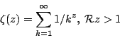 |
(30) |
Differentiation of equation 29
yields:
The end result of these calculations is that
What we have not proved here is that LN for the ``Poissonized coin toss'' is a good enough approximation to the longest run problem with exactly n coin tosses. However, this is not the application we are interested in.
Computer simulations of coin tossing.
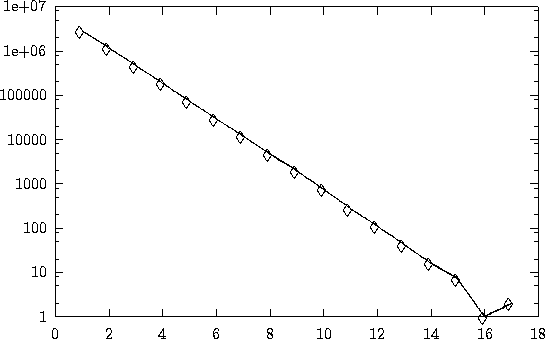
In 216 (65536) tosses of a fair coin, the computer generated 32659 heads and 32877 tails. There were 16400 runs of heads of size > 0. This and various other simulations gave results shown in Figures 1, 2, 3 and 4.
![\begin{figure}\setlength{\unitlength}{0.240900pt}
\ifx\plotpoint\undefined\ne...
...
\put(1256.0,68.0){\rule[-0.200pt]{43.362pt}{0.400pt}}
\end{picture}\end{figure}](Probability, runs, longest exact matches & gapless local alignment_files/img143.gif) |
Local alignment without gaps
Let's return to sequence alignment.
![]()
and ![]()
are 2 biomolecular sequences of the same
type (from the same alphabet). Let's refer to the alphabet as ![]() , where, for DNA, K=4 and
, where, for DNA, K=4 and ![]() . For proteins, K=20 and
. For proteins, K=20 and ![]()
S,T,V,W,Y}. This time, however, we will
regard the {ai} as i.i.d. random variables, and the same with
{bj}. Let p =
P(ai = bj). We do not
assume that the ais and bjs
have the same distribution. The degree to which they may differ is restricted,
and is beyond the scope of this course. For example, if P(ai
= Ah)P(bj =
Ah) = 0 for all members of the alphabet, then nothing
useful results.
 |
Let Lm,n be the largest non-negative integer,
k, such that there is some ![]() and some
and some ![]() such that
such that ![]() . In other words,
Lm,n is the ``longest run of exact matches''.
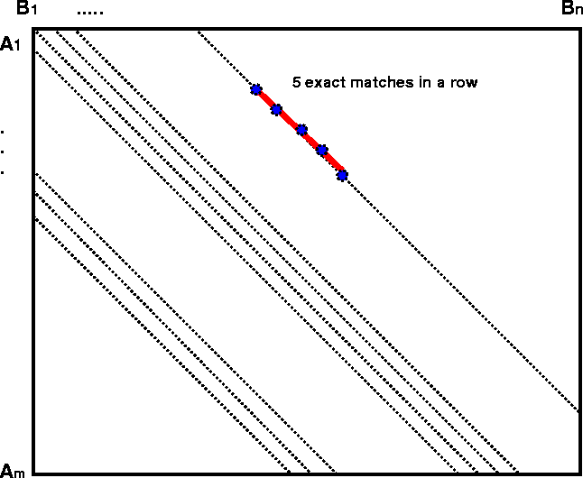
How is this problem similar to the ``longest run of heads matches'' in coin
tossing? We can think of the familiar m x n ``dot plot'' matrix,
where the ``blanks'' are ``tails'' and the ``dots'' are ``head''. Instead of a
linear array of coin tosses, we have a 2D grid and search for the maximum number
of dots in a row along successive diagonals, j-i = d, for
. In other words,
Lm,n is the ``longest run of exact matches''.
How is this problem similar to the ``longest run of heads matches'' in coin
tossing? We can think of the familiar m x n ``dot plot'' matrix,
where the ``blanks'' are ``tails'' and the ``dots'' are ``head''. Instead of a
linear array of coin tosses, we have a 2D grid and search for the maximum number
of dots in a row along successive diagonals, j-i = d, for ![]() . The total length of all these diagonals is
mn. Of course, the dots are not independent random variables, even though
they are independent of each other along any diagonal. Let
ph and p'h be
P(ai = Ah) and
P(bj = Ah),
respectively. Then
. The total length of all these diagonals is
mn. Of course, the dots are not independent random variables, even though
they are independent of each other along any diagonal. Let
ph and p'h be
P(ai = Ah) and
P(bj = Ah),
respectively. Then ![]() , so that
, so that ![]() , while P(ai=bj)P(ai+1=bj)
= p2. These 2 quantities will be unequal in general.
, while P(ai=bj)P(ai+1=bj)
= p2. These 2 quantities will be unequal in general.
It turns out that the non-independence of the dots on different diagonals and
the effect of stringing all the diagonals together into a long ``coin toss'' of
size mn doesn't make a lot of difference. The basic results hold for
large mn. That is ![]()
is an excellent approximation to ![]() and
and ![]() is an excellent approximation to
is an excellent approximation to ![]() .
.
Now we consider local alignment with a scoring function w. Note that
w(ai,bj) is now a
random variable. We will assume that ![]() , so that no gaps will be predicted. Let
H(m,n) be the maximum local alignment weight achieved by
aligning
, so that no gaps will be predicted. Let
H(m,n) be the maximum local alignment weight achieved by
aligning ![]() with
with ![]() .
.
We will now define sufficient conditions on w(ai,bj) so that H(m,n) behaves like the longest run in a coin toss.
Let ph =
P(ai = Ah) and p'h =
P(bj = Ah). Also, we'll
write wh1,h2 for the more cumbersome w(Ah1,Ah2).
Suppose that the match weights, ![]() satisfy:
satisfy:
Then ![]()
![\begin{figure}
\setlength{\unitlength}{0.240900pt}
\ifx\plotpoint\undefined\new...
...ut(1140.0,68.0){\rule[-0.400pt]{0.800pt}{194.888pt}}
\end{picture}
\end{figure}](Probability, runs, longest exact matches & gapless local alignment_files/img168.gif) |
Proof: Define ![]() .
.
Note that f(0) = 1. The negative
expected score assures that f'(0) < 0. Thus ![]() . The existence of h1' and h2' as
described ensures that
. The existence of h1' and h2' as
described ensures that ![]() . Thus
. Thus ![]() . The uniqueness of
. The uniqueness of ![]() follows from the fact that f'' > 0
(convex function).
follows from the fact that f'' > 0
(convex function).
An immediate consequence of this simple theorem is that we can define new
probabilities:
Recall equation 25. We
can rewrite it replacing ![]() with
with ![]() and derive:
and derive:
In comparison, Karlin showed that for the H(m,n)
statistic, with the weights satisfying the above conditions, there is another
constant, K* >0 such that
| Michael Zuker Professor of Mathematical Sciences Rensselaer Polytechnic Institute 2003-02-07 |


![$\displaystyle \rm {\bf E}[\sum_{i=1}^{N} (R'_i + 1])$](Probability, runs, longest exact matches & gapless local alignment_files/img111.gif)
![$\displaystyle e^{-qn} \sum_{j=1}^{\infty}
\frac{(nq)^j}{j!} j \rm {\bf E}[R'_i + 1]$](Probability, runs, longest exact matches & gapless local alignment_files/img112.gif)
![$\displaystyle \sum_{n=2}^{\infty}(-1)^{n}[\zeta(n)-1]z^{n}/n,$](Probability, runs, longest exact matches & gapless local alignment_files/img128.gif)

![$\displaystyle \sum_{n=2}^{\infty}(-1)^{n}[\zeta(n)-1]z^{n-1}.$](Probability, runs, longest exact matches & gapless local alignment_files/img136.gif)
![\begin{figure}\setlength{\unitlength}{0.240900pt}
\ifx\plotpoint\undefined\ne...
...
\put(1247.0,68.0){\rule[-0.200pt]{45.530pt}{0.400pt}}
\end{picture}\end{figure}](Probability, runs, longest exact matches & gapless local alignment_files/img144.gif)
![\begin{figure}\setlength{\unitlength}{0.240900pt}
\ifx\plotpoint\undefined\ne...
...
\put(1234.0,68.0){\rule[-0.200pt]{36.617pt}{0.400pt}}
\end{picture}\end{figure}](Probability, runs, longest exact matches & gapless local alignment_files/img145.gif)