Theoretical Quantile-Quantile Plots:
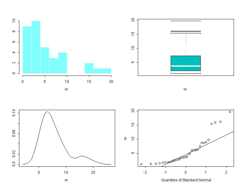
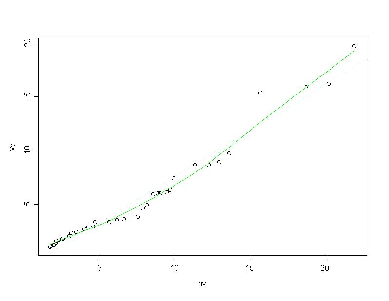
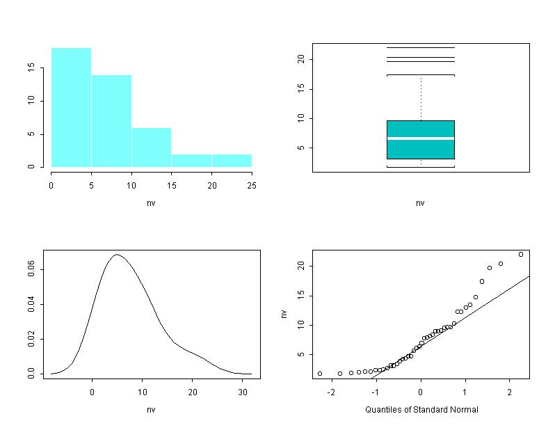
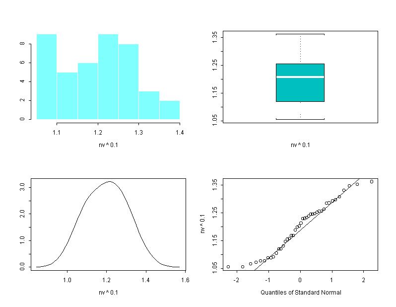
the stereogram dataset
"Length of time in seconds taken by subjects to see a three dimensional object, (a spiral ramp coming out of the page), in a random dot stereogram. The subjects were given varying prior information about the object; 42 receiving either no information or verbal information only (nv), and 35 receiving both verbal and visual information (vv). ... Data were digitalized from the article and rounded. Source: Frisby and Clatworthy (1975), [Chapter 6]."
|
|
|
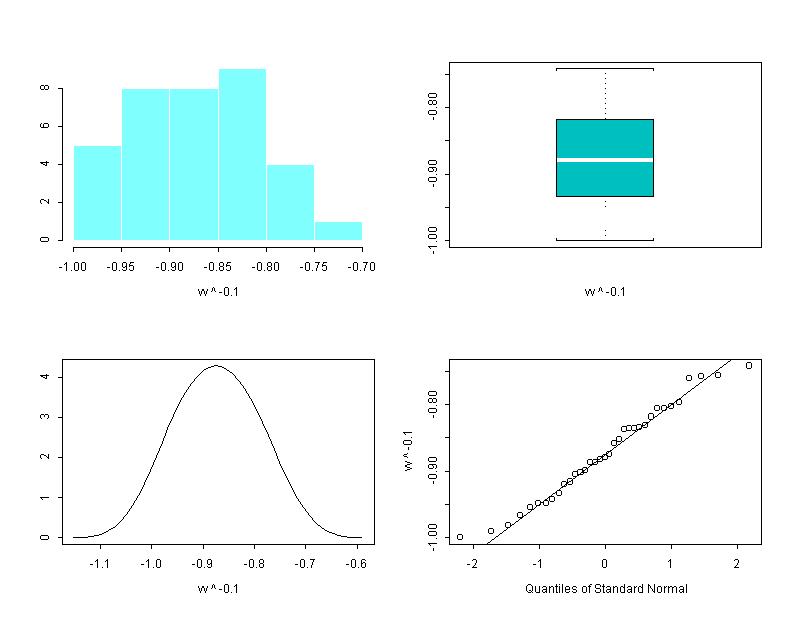
Note: here powernormal(x,theta) is defined as -(xtheta) if theta is negative (cf. GMDA, by Chambers et al, p214).
(A rightward shift is to be used if x assumes negative values. )
For another definition of powernormal(x,theta) see Visualizing Data, by Cleveland, p56, where
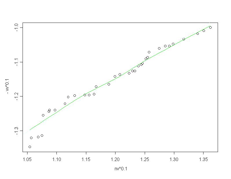
powernormal2(x,theta) is defined simply as xtheta for a negative theta.
[for negative theta both transformations reverse the upper and lower tails of the distribution]
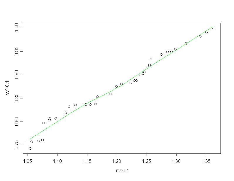
Quantile-quantile plot: powernormal2(vv,-0.1) vs. powernormal2(nv,0.1)