Problem Set 5: Key

Problem Set 5: Key

THE DOWNWARD SLOPE OF AD AND UPWARD SLOPE OF AS

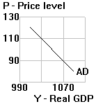
Consider the following information: investment (I) always equals $200, government purchases (G) $150, and net exports (X-M) $0. Use this information plus the consumption information in the table below to complete the aggregate demand (AD) row of the table.

Price level	80	90	100	110	120
Consumption	740	720	700	680	660
Aggregate demand	1090	1070	1050	1030	1010

Construct an aggregate demand (AD) curve. See diagram.

What accounts for the inverse relationship between consumption and the price level? Wealth effect: (Higher price level reduces value of money holdings --> save more and consume less to replenish wealth. So C falls.)

In general, what other reasons make the AD curve slope down? (1) Interest rate effect (Higher price level makes people hold onto more cash for their purchases, so they loan out less, driving up the interest rate which reduces investment (I) spending); and (2) International competitiveness effect (Higher domestic price level reduces international competitiveness, so buyers switch to foreign products. So X falls and M rises => (X-M) falls.)

Suppose you have signed a yearlong contract to pay a supplier $10 per unit for an item that you order and then resell with no additional costs involved.

Suppose that you can sell the item you order for $10 apiece when the economy's price level is at 100, and that your output price moves in exactly the same proportion as the price level. Compute your surplus (profit) per unit for each of the following possible price levels: 85, 100, 115, 130.

Price level	Output price	Input cost	Profit per unit
85	$ 8.50	$10.00	-$1.50
100	$10.00	$10.00	$0.00
115	$11.50	$10.00	$1.50
130	$13.00	$10.00	$3.00

How do the computations from part a help explain the upward slope of the short-run aggregate supply curve?
With fixed input cost, higher price level raises profits, encouraging sellers to produce more.

AD-AS ANALYSIS

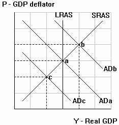
3.	Construct a diagram with SRAS and LRAS curves for an economy. Now add to your diagrams three AD curves to illustrate the following three possible short-run equilibrium situations for the economy: (1) a recession, (2) full employment and (3) an economic boom. In you diagram, clearly label the price level and real GDP for each of the three situations. See diagram. (1) c= recession; (2) a=Yf; (3) b=boom.

The following table contains hypothetical information about real GDP (billions of dollars) and the price level index (P):

AD	P	SRAS
$270	160	$330
290	140	310
310	120	290
330	100	270
350	80	250

Plot the data in an aggregate demand/aggregate supply diagram. What is the current equilibrium level of real GDP? The price level?
Y=300; P=130

What is the current value of nominal GDP? NGDP = 300x(130/100)=390

Suppose the level of full-employment real GDP is $320 billion. Add a LRAS curve to your diagram. See diagram to the right

Is this economy experiencing full employment, a recession, or a boom? How large? A recession: Y<Yf by $20B

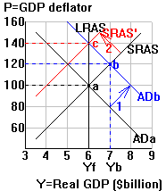
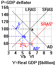
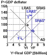
5.	a.	For each of the events below, begin by constructing an AD/SRAS/LRAS diagram which shows the U.S. economy in a full-employment equilibrium. Then use your diagram to depict the short-run effects of each of the following events on real GDP and the price level. Use a separate diagram for each event. a and b. See diagrams:
		(1)	Exports increase as the result of an unanticipated rapid growth of incomes abroad.
		(2)	Gloomy economic forecasts lead households to save more income for that "rainy day."
		(3)	A major new discovery of oil, a significant industrial input, occurs.
	b.	Now, illustrate what will eventually happen to the SRAS curve as a result of each of the three events (consider each event separately).

			(1)	(2)	(3)
		Note regarding b(3): If you shift LRAS and SRAS, then you might not need any self-correction. You need self-correction only if Yb doesn't equal Yf. If Yb>Yf, repeat b(1), if Yb<Yf, repeat b(2).

Consider the following information (consider each situation separately):

	Year	Actual real output	Full-employment output	Unemployment Rate	GDP deflator (2005=100)
	Year	(billions of 2005 dollars)		Unemployment Rate	GDP deflator (2005=100)
(1)	1933	$850	$1,120	24.9%	6.6
(2)	1969	3,664	3,616	3.8	20.6
(3)	1982	5,694	6,225	9.7	55.6
(4)	1997	9,550	9,550	5.0	84.6

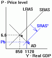
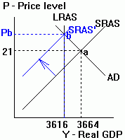
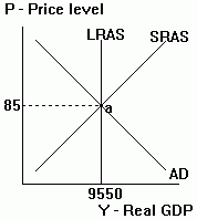
Depict each of the four years above in four separate aggregate demand/aggregate supply diagrams in which you show AD, SRAS and LRAS (=Yf), and the listed values of total output. See diagrams

(1) = 1933

(2) = 1969

(4) = 1988

Similar in (3) 1982, with P=56, Y=5694 and Yf=6225

Suppose the self-correction mechanism of the classical economy operates without impediment. Carefully explain how the self-correcting mechanism should have worked in (1) 1933, (2) 1969, and (3) 1982. Show the adjustments in your diagrams. (See Figures 27-5, 27-6 and 27-7 in the supplementary readings from Baumol and Blinder, "The Aggregate Supply Curve," as well as the discussion that accompanies the figures.)

    1933 and 1982: Y<Yf --. U>Uf => excess supply of resources --> resource suppliers bid down resource prices --> SRAS shifts down until Y=Yf again..
    1969: Y>Yf --> U<Uf => excess demand for resources --> firms bid up resource prices --> SRAS shifts up until Y=Yf again.
    1997: Y=Yf, so macro is in a long-run equilibrium.